>>> """
=======================
TickedStroke patheffect
=======================

Matplotlib's :mod:`.patheffects` can be used to alter the way paths
are drawn at a low enough level that they can affect almost anything.

The :doc:`patheffects guide</tutorials/advanced/patheffects_guide>`
details the use of patheffects.

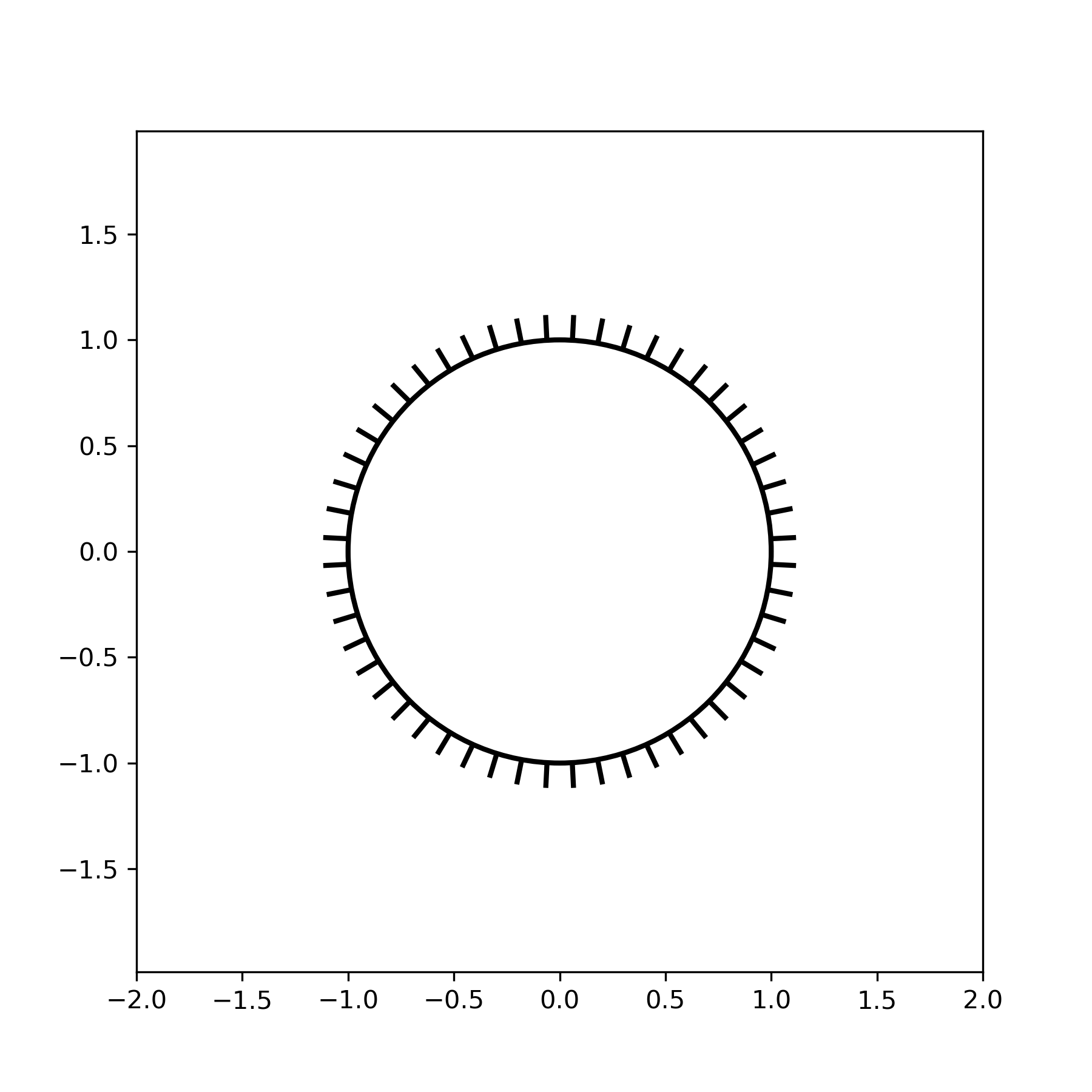
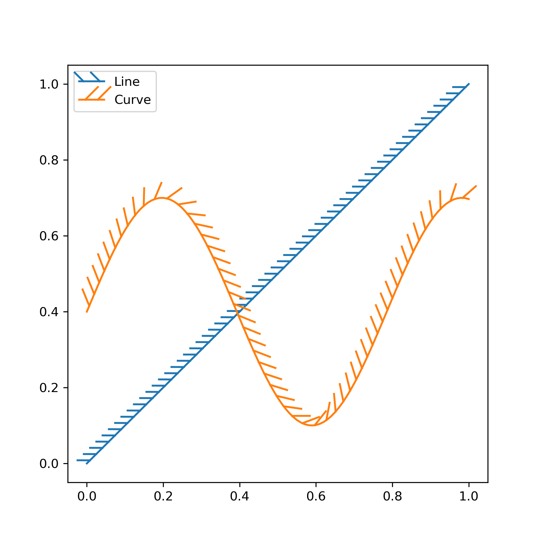
The `~matplotlib.patheffects.TickedStroke` patheffect illustrated here
draws a path with a ticked style.  The spacing, length, and angle of
ticks can be controlled.

See also the :doc:`contour demo example
</gallery/lines_bars_and_markers/lines_with_ticks_demo>`.

See also the :doc:`contours in optimization example
</gallery/images_contours_and_fields/contours_in_optimization_demo>`.
"""
... 
... ###############################################################################
... # Applying TickedStroke to paths
... # ==============================
... import matplotlib.patches as patches
... from matplotlib.path import Path
... import numpy as np
... import matplotlib.pyplot as plt
... import matplotlib.patheffects as patheffects
... 
... fig, ax = plt.subplots(figsize=(6, 6))
... path = Path.unit_circle()
... patch = patches.PathPatch(path, facecolor='none', lw=2, path_effects=[
...     patheffects.withTickedStroke(angle=-90, spacing=10, length=1)])
... 
... ax.add_patch(patch)
... ax.axis('equal')
... ax.set_xlim(-2, 2)
... ax.set_ylim(-2, 2)
... 
... plt.show()
... 
... ###############################################################################
... # Applying TickedStroke to lines
... # ==============================
... fig, ax = plt.subplots(figsize=(6, 6))
... ax.plot([0, 1], [0, 1], label="Line",
...         path_effects=[patheffects.withTickedStroke(spacing=7, angle=135)])
... 
... nx = 101
... x = np.linspace(0.0, 1.0, nx)
... y = 0.3*np.sin(x*8) + 0.4
... ax.plot(x, y, label="Curve", path_effects=[patheffects.withTickedStroke()])
... 
... ax.legend()
... 
... plt.show()
... 
... ###############################################################################
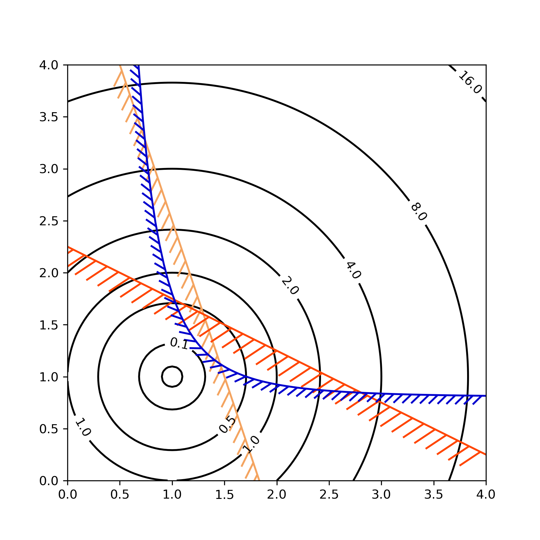
... # Applying TickedStroke to contour plots
... # ======================================
... #
... # Contour plot with objective and constraints.
... # Curves generated by contour to represent a typical constraint in an
... # optimization problem should be plotted with angles between zero and
... # 180 degrees.
... fig, ax = plt.subplots(figsize=(6, 6))
... 
... nx = 101
... ny = 105
... 
... # Set up survey vectors
... xvec = np.linspace(0.001, 4.0, nx)
... yvec = np.linspace(0.001, 4.0, ny)
... 
... # Set up survey matrices.  Design disk loading and gear ratio.
... x1, x2 = np.meshgrid(xvec, yvec)
... 
... # Evaluate some stuff to plot
... obj = x1**2 + x2**2 - 2*x1 - 2*x2 + 2
... g1 = -(3*x1 + x2 - 5.5)
... g2 = -(x1 + 2*x2 - 4.5)
... g3 = 0.8 + x1**-3 - x2
... 
... cntr = ax.contour(x1, x2, obj, [0.01, 0.1, 0.5, 1, 2, 4, 8, 16],
...                   colors='black')
... ax.clabel(cntr, fmt="%2.1f", use_clabeltext=True)
... 
... cg1 = ax.contour(x1, x2, g1, [0], colors='sandybrown')
... plt.setp(cg1.collections,
...          path_effects=[patheffects.withTickedStroke(angle=135)])
... 
... cg2 = ax.contour(x1, x2, g2, [0], colors='orangered')
... plt.setp(cg2.collections,
...          path_effects=[patheffects.withTickedStroke(angle=60, length=2)])
... 
... cg3 = ax.contour(x1, x2, g3, [0], colors='mediumblue')
... plt.setp(cg3.collections,
...          path_effects=[patheffects.withTickedStroke(spacing=7)])
... 
... ax.set_xlim(0, 4)
... ax.set_ylim(0, 4)
... 
... plt.show()
...