>>> """
==============
Secondary Axis
==============

Sometimes we want a secondary axis on a plot, for instance to convert
radians to degrees on the same plot.  We can do this by making a child
axes with only one axis visible via `.axes.Axes.secondary_xaxis` and
`.axes.Axes.secondary_yaxis`.  This secondary axis can have a different scale
than the main axis by providing both a forward and an inverse conversion
function in a tuple to the *functions* keyword argument:
"""
... 
... import matplotlib.pyplot as plt
... import numpy as np
... import datetime
... import matplotlib.dates as mdates
... from matplotlib.ticker import AutoMinorLocator
... 
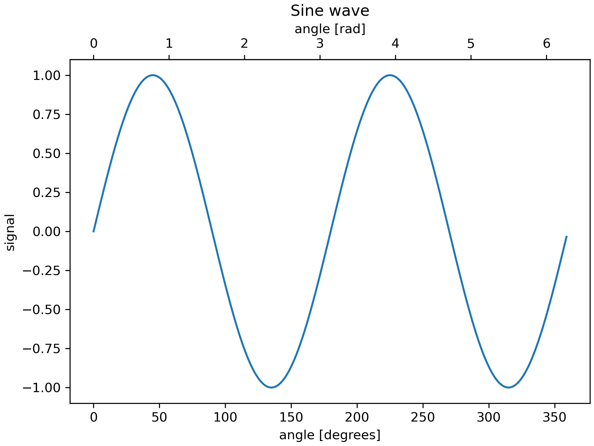
... fig, ax = plt.subplots(constrained_layout=True)
... x = np.arange(0, 360, 1)
... y = np.sin(2 * x * np.pi / 180)
... ax.plot(x, y)
... ax.set_xlabel('angle [degrees]')
... ax.set_ylabel('signal')
... ax.set_title('Sine wave')
... 
... 
... def deg2rad(x):
...     return x * np.pi / 180
... 
... 
... def rad2deg(x):
...     return x * 180 / np.pi
... 
... 
... secax = ax.secondary_xaxis('top', functions=(deg2rad, rad2deg))
... secax.set_xlabel('angle [rad]')
... plt.show()
... 
... ###########################################################################
... # Here is the case of converting from wavenumber to wavelength in a
... # log-log scale.
... #
... # .. note::
... #
... #   In this case, the xscale of the parent is logarithmic, so the child is
... #   made logarithmic as well.
... 
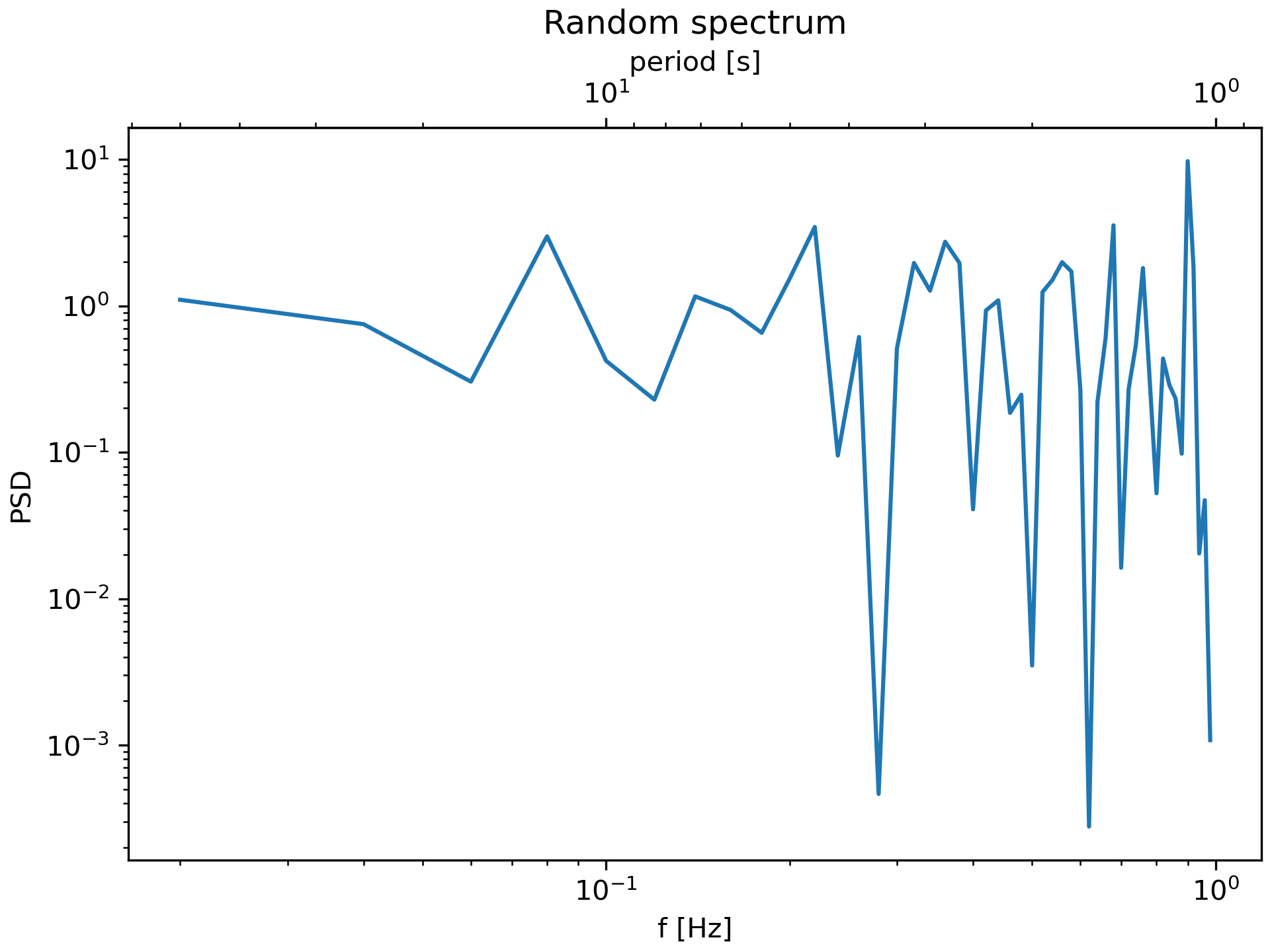
... fig, ax = plt.subplots(constrained_layout=True)
... x = np.arange(0.02, 1, 0.02)
... np.random.seed(19680801)
... y = np.random.randn(len(x)) ** 2
... ax.loglog(x, y)
... ax.set_xlabel('f [Hz]')
... ax.set_ylabel('PSD')
... ax.set_title('Random spectrum')
... 
... 
... def one_over(x):
...     """Vectorized 1/x, treating x==0 manually"""
...     x = np.array(x).astype(float)
...     near_zero = np.isclose(x, 0)
...     x[near_zero] = np.inf
...     x[~near_zero] = 1 / x[~near_zero]
...     return x
... 
... 
... # the function "1/x" is its own inverse
... inverse = one_over
... 
... 
... secax = ax.secondary_xaxis('top', functions=(one_over, inverse))
... secax.set_xlabel('period [s]')
... plt.show()
... 
... ###########################################################################
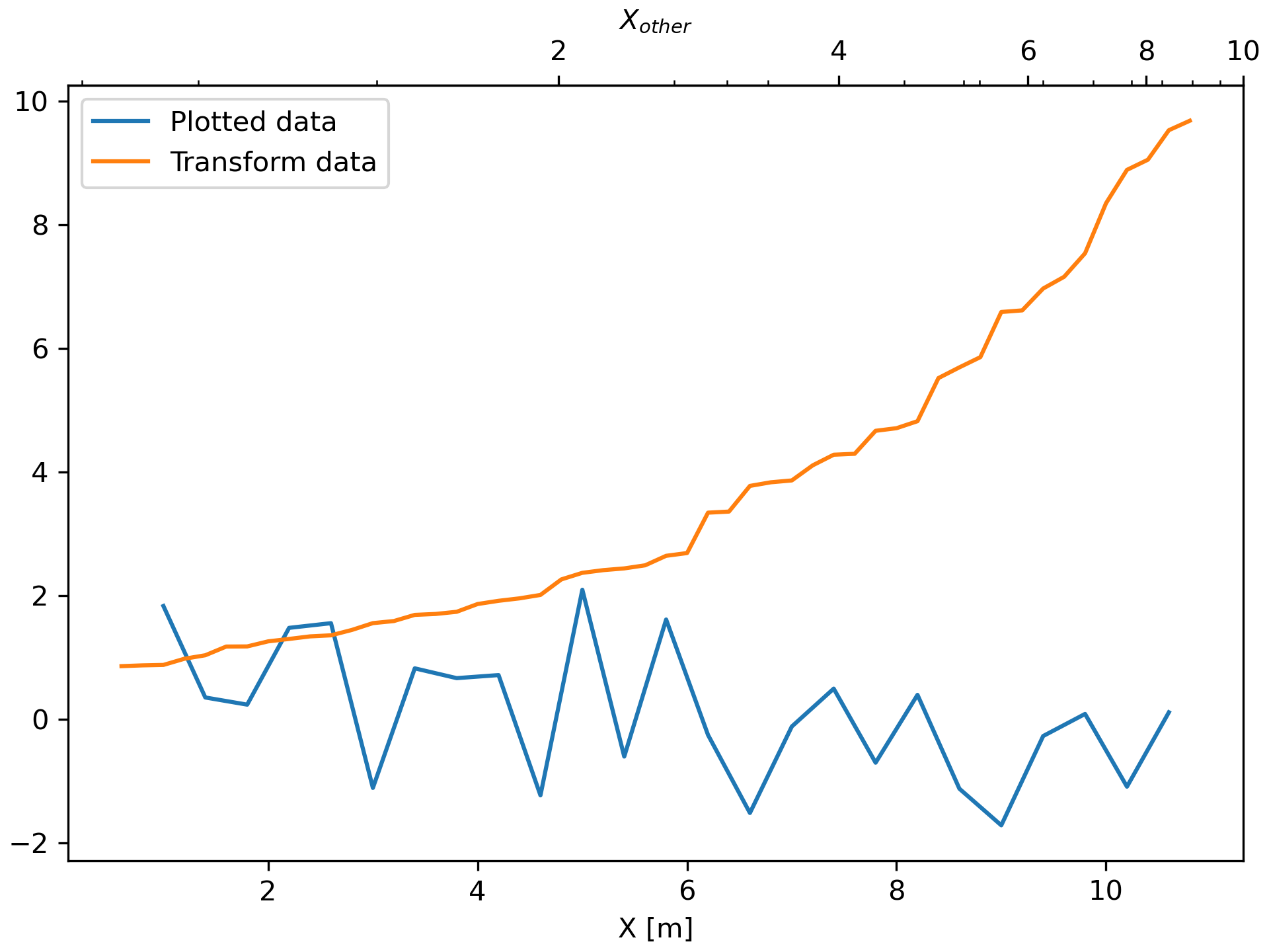
... # Sometime we want to relate the axes in a transform that is ad-hoc from
... # the data, and is derived empirically.  In that case we can set the
... # forward and inverse transforms functions to be linear interpolations from the
... # one data set to the other.
... #
... # .. note::
... #
... #   In order to properly handle the data margins, the mapping functions
... #   (``forward`` and ``inverse`` in this example) need to be defined beyond the
... #   nominal plot limits.
... #
... #   In the specific case of the numpy linear interpolation, `numpy.interp`,
... #   this condition can be arbitrarily enforced by providing optional keyword
... #   arguments *left*, *right* such that values outside the data range are
... #   mapped well outside the plot limits.
... 
... fig, ax = plt.subplots(constrained_layout=True)
... xdata = np.arange(1, 11, 0.4)
... ydata = np.random.randn(len(xdata))
... ax.plot(xdata, ydata, label='Plotted data')
... 
... xold = np.arange(0, 11, 0.2)
... # fake data set relating x coordinate to another data-derived coordinate.
... # xnew must be monotonic, so we sort...
... xnew = np.sort(10 * np.exp(-xold / 4) + np.random.randn(len(xold)) / 3)
... 
... ax.plot(xold[3:], xnew[3:], label='Transform data')
... ax.set_xlabel('X [m]')
... ax.legend()
... 
... 
... def forward(x):
...     return np.interp(x, xold, xnew)
... 
... 
... def inverse(x):
...     return np.interp(x, xnew, xold)
... 
... 
... secax = ax.secondary_xaxis('top', functions=(forward, inverse))
... secax.xaxis.set_minor_locator(AutoMinorLocator())
... secax.set_xlabel('$X_{other}$')
... 
... plt.show()
... 
... ###########################################################################
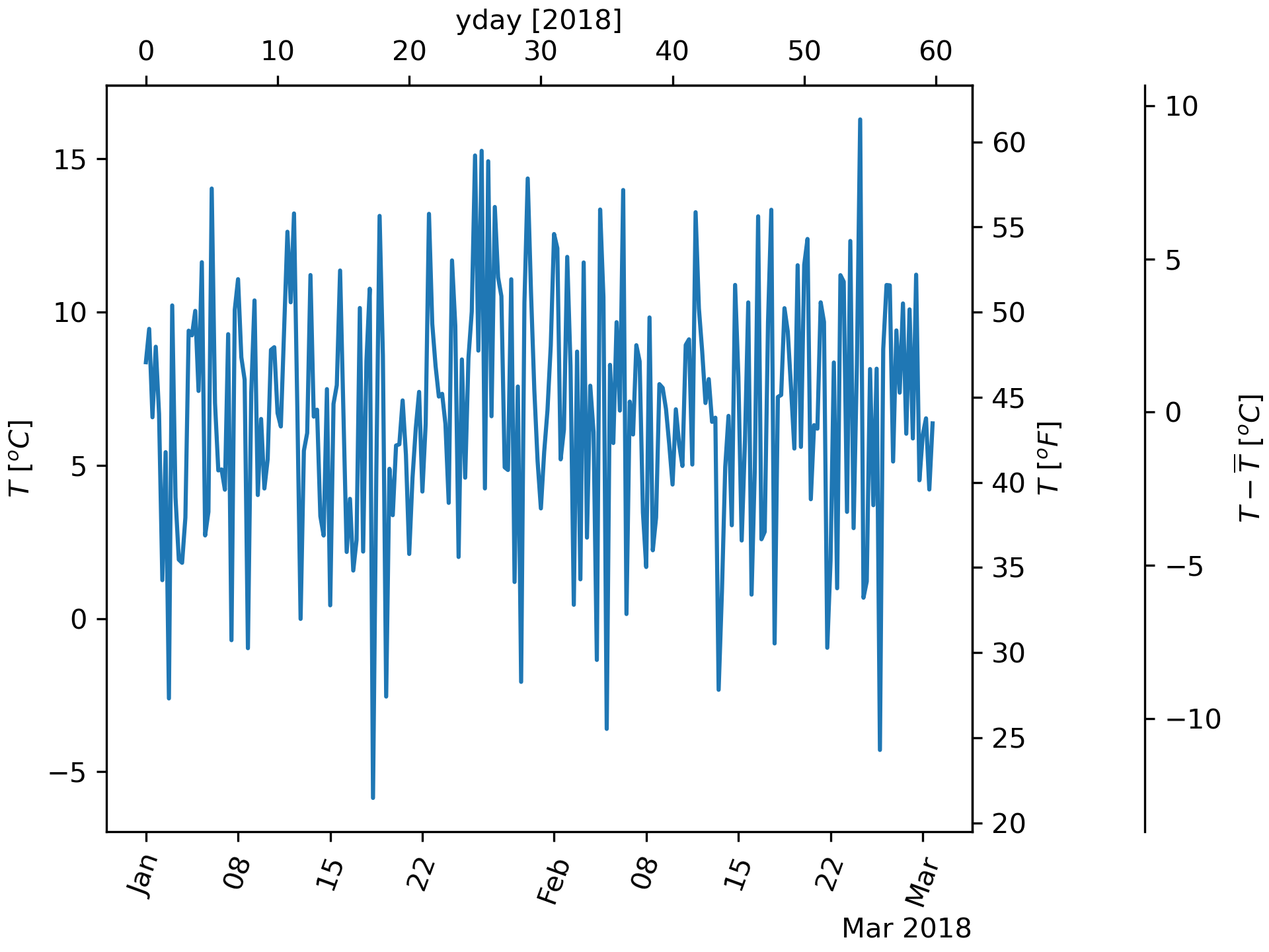
... # A final example translates np.datetime64 to yearday on the x axis and
... # from Celsius to Fahrenheit on the y axis.  Note the addition of a
... # third y axis, and that it can be placed using a float for the
... # location argument
... 
... dates = [datetime.datetime(2018, 1, 1) + datetime.timedelta(hours=k * 6)
...          for k in range(240)]
... temperature = np.random.randn(len(dates)) * 4 + 6.7
... fig, ax = plt.subplots(constrained_layout=True)
... 
... ax.plot(dates, temperature)
... ax.set_ylabel(r'$T\ [^oC]$')
... plt.xticks(rotation=70)
... 
... 
... def date2yday(x):
...     """Convert matplotlib datenum to days since 2018-01-01."""
...     y = x - mdates.date2num(datetime.datetime(2018, 1, 1))
...     return y
... 
... 
... def yday2date(x):
...     """Return a matplotlib datenum for *x* days after 2018-01-01."""
...     y = x + mdates.date2num(datetime.datetime(2018, 1, 1))
...     return y
... 
... 
... secax_x = ax.secondary_xaxis('top', functions=(date2yday, yday2date))
... secax_x.set_xlabel('yday [2018]')
... 
... 
... def celsius_to_fahrenheit(x):
...     return x * 1.8 + 32
... 
... 
... def fahrenheit_to_celsius(x):
...     return (x - 32) / 1.8
... 
... 
... secax_y = ax.secondary_yaxis(
...     'right', functions=(celsius_to_fahrenheit, fahrenheit_to_celsius))
... secax_y.set_ylabel(r'$T\ [^oF]$')
... 
... 
... def celsius_to_anomaly(x):
...     return (x - np.mean(temperature))
... 
... 
... def anomaly_to_celsius(x):
...     return (x + np.mean(temperature))
... 
... 
... # use of a float for the position:
... secax_y2 = ax.secondary_yaxis(
...     1.2, functions=(celsius_to_anomaly, anomaly_to_celsius))
... secax_y2.set_ylabel(r'$T - \overline{T}\ [^oC]$')
... 
... 
... plt.show()
... 
... #############################################################################
... #
... # .. admonition:: References
... #
... #    The use of the following functions, methods, classes and modules is shown
... #    in this example:
... #
... #    - `matplotlib.axes.Axes.secondary_xaxis`
... #    - `matplotlib.axes.Axes.secondary_yaxis`
...