>>> """
================
The Sankey class
================

Demonstrate the Sankey class by producing three basic diagrams.
"""
... 
... import matplotlib.pyplot as plt
... 
... from matplotlib.sankey import Sankey
... 
... 
... ###############################################################################
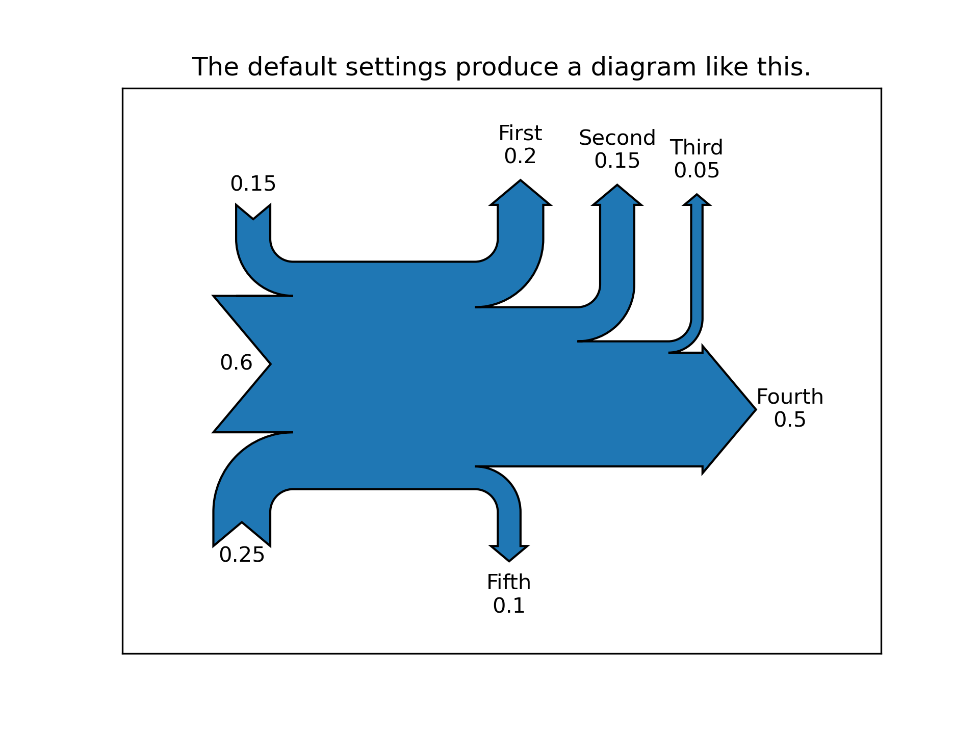
... # Example 1 -- Mostly defaults
... #
... # This demonstrates how to create a simple diagram by implicitly calling the
... # Sankey.add() method and by appending finish() to the call to the class.
... 
... Sankey(flows=[0.25, 0.15, 0.60, -0.20, -0.15, -0.05, -0.50, -0.10],
...        labels=['', '', '', 'First', 'Second', 'Third', 'Fourth', 'Fifth'],
...        orientations=[-1, 1, 0, 1, 1, 1, 0, -1]).finish()
... plt.title("The default settings produce a diagram like this.")
... 
... ###############################################################################
... # Notice:
... #
... # 1. Axes weren't provided when Sankey() was instantiated, so they were
... #    created automatically.
... # 2. The scale argument wasn't necessary since the data was already
... #    normalized.
... # 3. By default, the lengths of the paths are justified.
... 
... 
... ###############################################################################
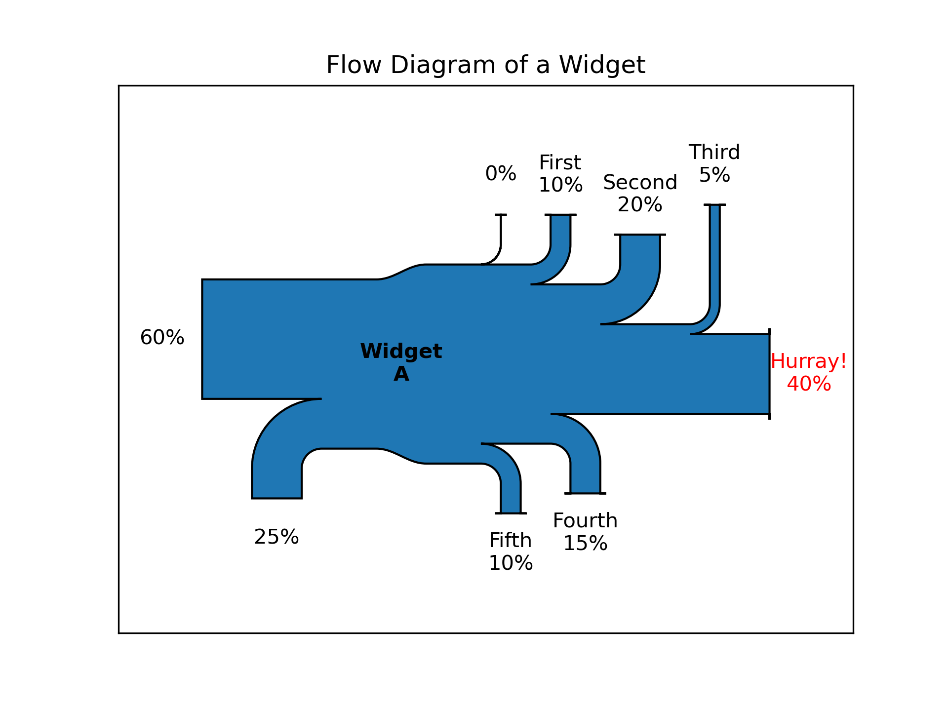
... # Example 2
... #
... # This demonstrates:
... #
... # 1. Setting one path longer than the others
... # 2. Placing a label in the middle of the diagram
... # 3. Using the scale argument to normalize the flows
... # 4. Implicitly passing keyword arguments to PathPatch()
... # 5. Changing the angle of the arrow heads
... # 6. Changing the offset between the tips of the paths and their labels
... # 7. Formatting the numbers in the path labels and the associated unit
... # 8. Changing the appearance of the patch and the labels after the figure is
... #    created
... 
... fig = plt.figure()
... ax = fig.add_subplot(1, 1, 1, xticks=[], yticks=[],
...                      title="Flow Diagram of a Widget")
... sankey = Sankey(ax=ax, scale=0.01, offset=0.2, head_angle=180,
...                 format='%.0f', unit='%')
... sankey.add(flows=[25, 0, 60, -10, -20, -5, -15, -10, -40],
...            labels=['', '', '', 'First', 'Second', 'Third', 'Fourth',
...                    'Fifth', 'Hurray!'],
...            orientations=[-1, 1, 0, 1, 1, 1, -1, -1, 0],
...            pathlengths=[0.25, 0.25, 0.25, 0.25, 0.25, 0.6, 0.25, 0.25,
...                         0.25],
...            patchlabel="Widget\nA")  # Arguments to matplotlib.patches.PathPatch
... diagrams = sankey.finish()
... diagrams[0].texts[-1].set_color('r')
... diagrams[0].text.set_fontweight('bold')
... 
... ###############################################################################
... # Notice:
... #
... # 1. Since the sum of the flows is nonzero, the width of the trunk isn't
... #    uniform.  The matplotlib logging system logs this at the DEBUG level.
... # 2. The second flow doesn't appear because its value is zero.  Again, this is
... #    logged at the DEBUG level.
... 
... 
... ###############################################################################
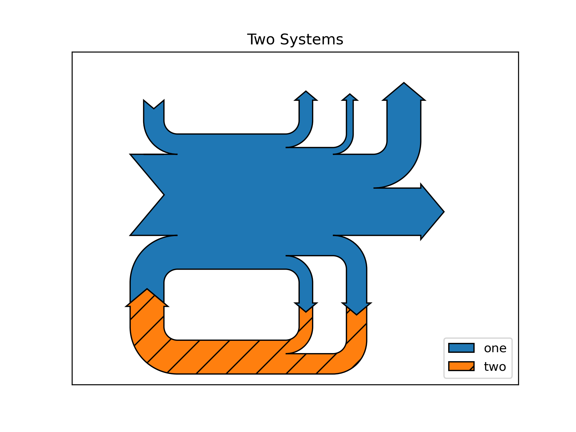
... # Example 3
... #
... # This demonstrates:
... #
... # 1. Connecting two systems
... # 2. Turning off the labels of the quantities
... # 3. Adding a legend
... 
... fig = plt.figure()
... ax = fig.add_subplot(1, 1, 1, xticks=[], yticks=[], title="Two Systems")
... flows = [0.25, 0.15, 0.60, -0.10, -0.05, -0.25, -0.15, -0.10, -0.35]
... sankey = Sankey(ax=ax, unit=None)
... sankey.add(flows=flows, label='one',
...            orientations=[-1, 1, 0, 1, 1, 1, -1, -1, 0])
... sankey.add(flows=[-0.25, 0.15, 0.1], label='two',
...            orientations=[-1, -1, -1], prior=0, connect=(0, 0))
... diagrams = sankey.finish()
... diagrams[-1].patch.set_hatch('/')
... plt.legend()
... 
... ###############################################################################
... # Notice that only one connection is specified, but the systems form a
... # circuit since: (1) the lengths of the paths are justified and (2) the
... # orientation and ordering of the flows is mirrored.
... 
... plt.show()
... 
... 
... #############################################################################
... #
... # .. admonition:: References
... #
... #    The use of the following functions, methods, classes and modules is shown
... #    in this example:
... #
... #    - `matplotlib.sankey`
... #    - `matplotlib.sankey.Sankey`
... #    - `matplotlib.sankey.Sankey.add`
... #    - `matplotlib.sankey.Sankey.finish`
...