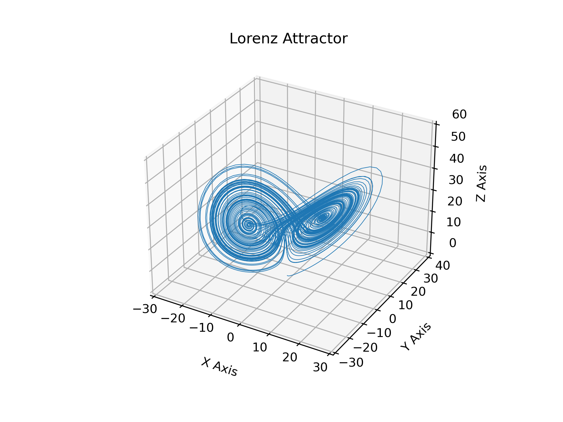
>>> """
================
Lorenz Attractor
================

This is an example of plotting Edward Lorenz's 1963 `"Deterministic Nonperiodic
Flow"`_ in a 3-dimensional space using mplot3d.

.. _"Deterministic Nonperiodic Flow":
   https://journals.ametsoc.org/view/journals/atsc/20/2/1520-0469_1963_020_0130_dnf_2_0_co_2.xml

.. note::
   Because this is a simple non-linear ODE, it would be more easily done using
   SciPy's ODE solver, but this approach depends only upon NumPy.
"""
... 
... import numpy as np
... import matplotlib.pyplot as plt
... 
... 
... def lorenz(x, y, z, s=10, r=28, b=2.667):
...     """
    Given:
       x, y, z: a point of interest in three dimensional space
       s, r, b: parameters defining the lorenz attractor
    Returns:
       x_dot, y_dot, z_dot: values of the lorenz attractor's partial
           derivatives at the point x, y, z
    """
...     x_dot = s*(y - x)
...     y_dot = r*x - y - x*z
...     z_dot = x*y - b*z
...     return x_dot, y_dot, z_dot
... 
... 
... dt = 0.01
... num_steps = 10000
... 
... # Need one more for the initial values
... xs = np.empty(num_steps + 1)
... ys = np.empty(num_steps + 1)
... zs = np.empty(num_steps + 1)
... 
... # Set initial values
... xs[0], ys[0], zs[0] = (0., 1., 1.05)
... 
... # Step through "time", calculating the partial derivatives at the current point
... # and using them to estimate the next point
... for i in range(num_steps):
...     x_dot, y_dot, z_dot = lorenz(xs[i], ys[i], zs[i])
...     xs[i + 1] = xs[i] + (x_dot * dt)
...     ys[i + 1] = ys[i] + (y_dot * dt)
...     zs[i + 1] = zs[i] + (z_dot * dt)
... 
... 
... # Plot
... ax = plt.figure().add_subplot(projection='3d')
... 
... ax.plot(xs, ys, zs, lw=0.5)
... ax.set_xlabel("X Axis")
... ax.set_ylabel("Y Axis")
... ax.set_zlabel("Z Axis")
... ax.set_title("Lorenz Attractor")
... 
... plt.show()
...