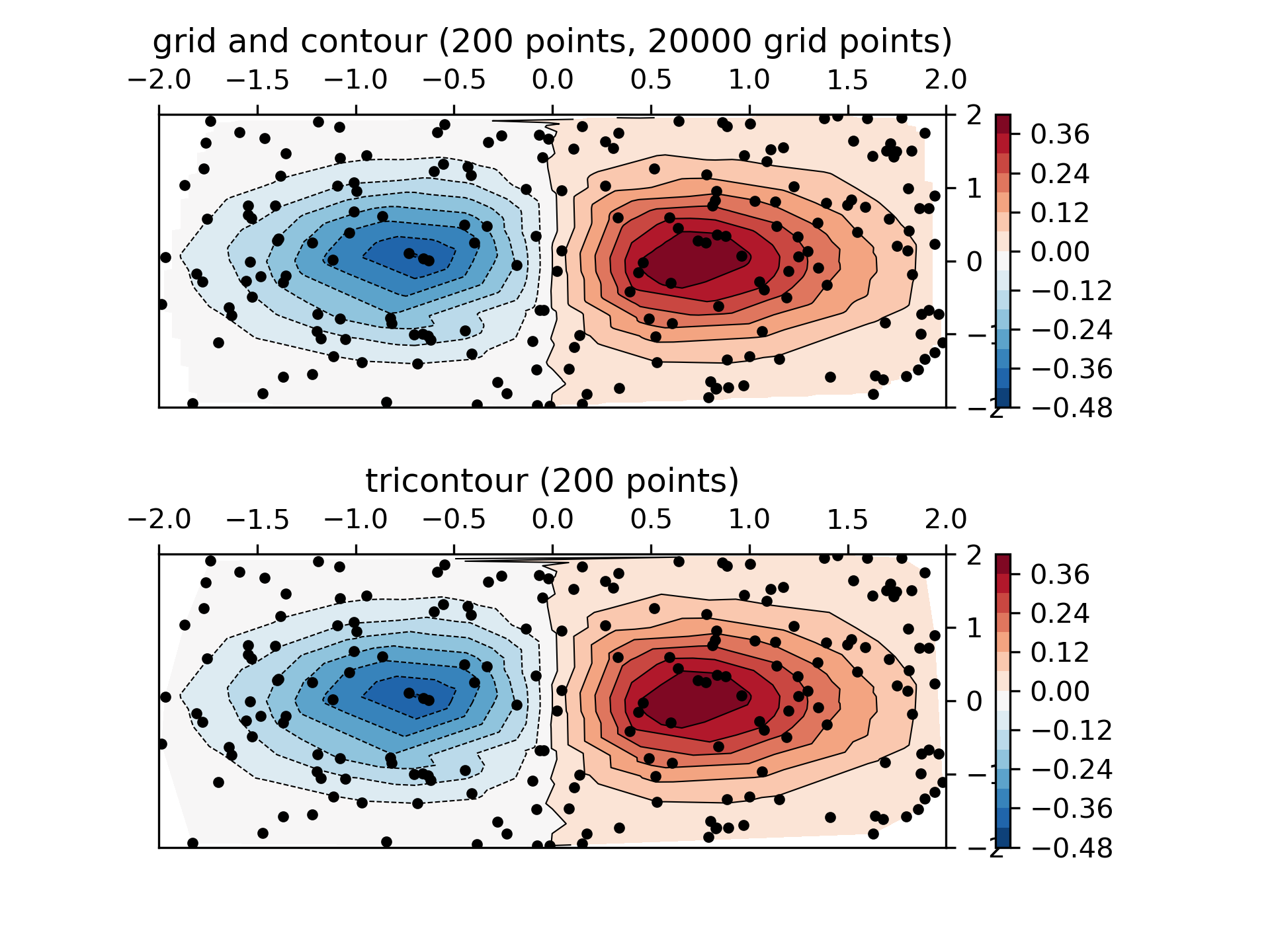
>>> """
=======================================
Contour plot of irregularly spaced data
=======================================

Comparison of a contour plot of irregularly spaced data interpolated
on a regular grid versus a tricontour plot for an unstructured triangular grid.

Since `~.axes.Axes.contour` and `~.axes.Axes.contourf` expect the data to live
on a regular grid, plotting a contour plot of irregularly spaced data requires
different methods. The two options are:

* Interpolate the data to a regular grid first. This can be done with on-board
  means, e.g. via `~.tri.LinearTriInterpolator` or using external functionality
  e.g. via `scipy.interpolate.griddata`. Then plot the interpolated data with
  the usual `~.axes.Axes.contour`.
* Directly use `~.axes.Axes.tricontour` or `~.axes.Axes.tricontourf` which will
  perform a triangulation internally.

This example shows both methods in action.
"""
... 
... import matplotlib.pyplot as plt
... import matplotlib.tri as tri
... import numpy as np
... 
... np.random.seed(19680801)
... npts = 200
... ngridx = 100
... ngridy = 200
... x = np.random.uniform(-2, 2, npts)
... y = np.random.uniform(-2, 2, npts)
... z = x * np.exp(-x**2 - y**2)
... 
... fig, (ax1, ax2) = plt.subplots(nrows=2)
... 
... # -----------------------
... # Interpolation on a grid
... # -----------------------
... # A contour plot of irregularly spaced data coordinates
... # via interpolation on a grid.
... 
... # Create grid values first.
... xi = np.linspace(-2.1, 2.1, ngridx)
... yi = np.linspace(-2.1, 2.1, ngridy)
... 
... # Linearly interpolate the data (x, y) on a grid defined by (xi, yi).
... triang = tri.Triangulation(x, y)
... interpolator = tri.LinearTriInterpolator(triang, z)
... Xi, Yi = np.meshgrid(xi, yi)
... zi = interpolator(Xi, Yi)
... 
... # Note that scipy.interpolate provides means to interpolate data on a grid
... # as well. The following would be an alternative to the four lines above:
... # from scipy.interpolate import griddata
... # zi = griddata((x, y), z, (xi[None, :], yi[:, None]), method='linear')
... 
... ax1.contour(xi, yi, zi, levels=14, linewidths=0.5, colors='k')
... cntr1 = ax1.contourf(xi, yi, zi, levels=14, cmap="RdBu_r")
... 
... fig.colorbar(cntr1, ax=ax1)
... ax1.plot(x, y, 'ko', ms=3)
... ax1.set(xlim=(-2, 2), ylim=(-2, 2))
... ax1.set_title('grid and contour (%d points, %d grid points)' %
...               (npts, ngridx * ngridy))
... 
... # ----------
... # Tricontour
... # ----------
... # Directly supply the unordered, irregularly spaced coordinates
... # to tricontour.
... 
... ax2.tricontour(x, y, z, levels=14, linewidths=0.5, colors='k')
... cntr2 = ax2.tricontourf(x, y, z, levels=14, cmap="RdBu_r")
... 
... fig.colorbar(cntr2, ax=ax2)
... ax2.plot(x, y, 'ko', ms=3)
... ax2.set(xlim=(-2, 2), ylim=(-2, 2))
... ax2.set_title('tricontour (%d points)' % npts)
... 
... plt.subplots_adjust(hspace=0.5)
... plt.show()
... 
... #############################################################################
... #
... # .. admonition:: References
... #
... #    The use of the following functions, methods, classes and modules is shown
... #    in this example:
... #
... #    - `matplotlib.axes.Axes.contour` / `matplotlib.pyplot.contour`
... #    - `matplotlib.axes.Axes.contourf` / `matplotlib.pyplot.contourf`
... #    - `matplotlib.axes.Axes.tricontour` / `matplotlib.pyplot.tricontour`
... #    - `matplotlib.axes.Axes.tricontourf` / `matplotlib.pyplot.tricontourf`
...