>>> """
Fill Between and Alpha
======================

The `~matplotlib.axes.Axes.fill_between` function generates a shaded
region between a min and max boundary that is useful for illustrating ranges.
It has a very handy ``where`` argument to combine filling with logical ranges,
e.g., to just fill in a curve over some threshold value.

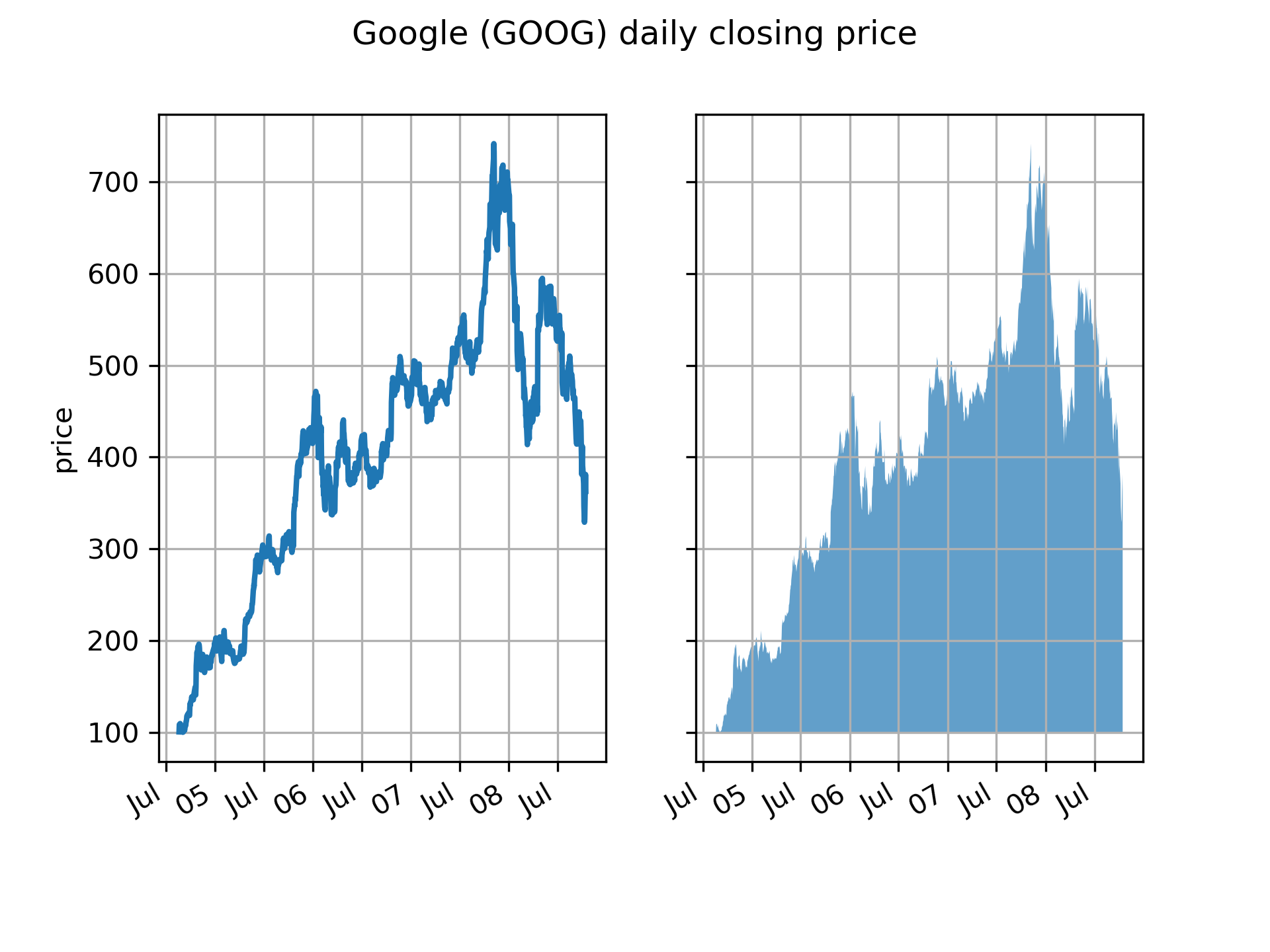
At its most basic level, ``fill_between`` can be use to enhance a graphs visual
appearance. Let's compare two graphs of a financial times with a simple line
plot on the left and a filled line on the right.
"""
... 
... import matplotlib.pyplot as plt
... import numpy as np
... import matplotlib.cbook as cbook
... 
... 
... # load up some sample financial data
... r = (cbook.get_sample_data('goog.npz', np_load=True)['price_data']
...      .view(np.recarray))
... # create two subplots with the shared x and y axes
... fig, (ax1, ax2) = plt.subplots(1, 2, sharex=True, sharey=True)
... 
... pricemin = r.close.min()
... 
... ax1.plot(r.date, r.close, lw=2)
... ax2.fill_between(r.date, pricemin, r.close, alpha=0.7)
... 
... for ax in ax1, ax2:
...     ax.grid(True)
... 
... ax1.set_ylabel('price')
... for label in ax2.get_yticklabels():
...     label.set_visible(False)
... 
... fig.suptitle('Google (GOOG) daily closing price')
... fig.autofmt_xdate()
... 
... ###############################################################################
... # The alpha channel is not necessary here, but it can be used to soften
... # colors for more visually appealing plots.  In other examples, as we'll
... # see below, the alpha channel is functionally useful as the shaded
... # regions can overlap and alpha allows you to see both.  Note that the
... # postscript format does not support alpha (this is a postscript
... # limitation, not a matplotlib limitation), so when using alpha save
... # your figures in PNG, PDF or SVG.
... #
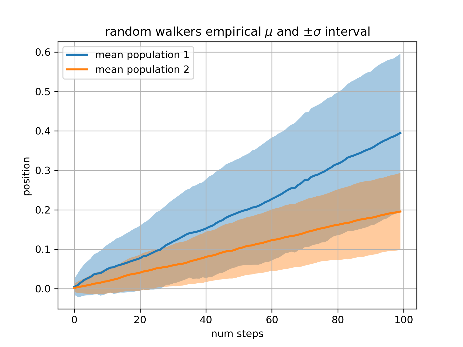
... # Our next example computes two populations of random walkers with a
... # different mean and standard deviation of the normal distributions from
... # which the steps are drawn.  We use filled regions to plot +/- one
... # standard deviation of the mean position of the population.  Here the
... # alpha channel is useful, not just aesthetic.
... 
... # Fixing random state for reproducibility
... np.random.seed(19680801)
... 
... Nsteps, Nwalkers = 100, 250
... t = np.arange(Nsteps)
... 
... # an (Nsteps x Nwalkers) array of random walk steps
... S1 = 0.004 + 0.02*np.random.randn(Nsteps, Nwalkers)
... S2 = 0.002 + 0.01*np.random.randn(Nsteps, Nwalkers)
... 
... # an (Nsteps x Nwalkers) array of random walker positions
... X1 = S1.cumsum(axis=0)
... X2 = S2.cumsum(axis=0)
... 
... 
... # Nsteps length arrays empirical means and standard deviations of both
... # populations over time
... mu1 = X1.mean(axis=1)
... sigma1 = X1.std(axis=1)
... mu2 = X2.mean(axis=1)
... sigma2 = X2.std(axis=1)
... 
... # plot it!
... fig, ax = plt.subplots(1)
... ax.plot(t, mu1, lw=2, label='mean population 1')
... ax.plot(t, mu2, lw=2, label='mean population 2')
... ax.fill_between(t, mu1+sigma1, mu1-sigma1, facecolor='C0', alpha=0.4)
... ax.fill_between(t, mu2+sigma2, mu2-sigma2, facecolor='C1', alpha=0.4)
... ax.set_title(r'random walkers empirical $\mu$ and $\pm \sigma$ interval')
... ax.legend(loc='upper left')
... ax.set_xlabel('num steps')
... ax.set_ylabel('position')
... ax.grid()
... 
... ###############################################################################
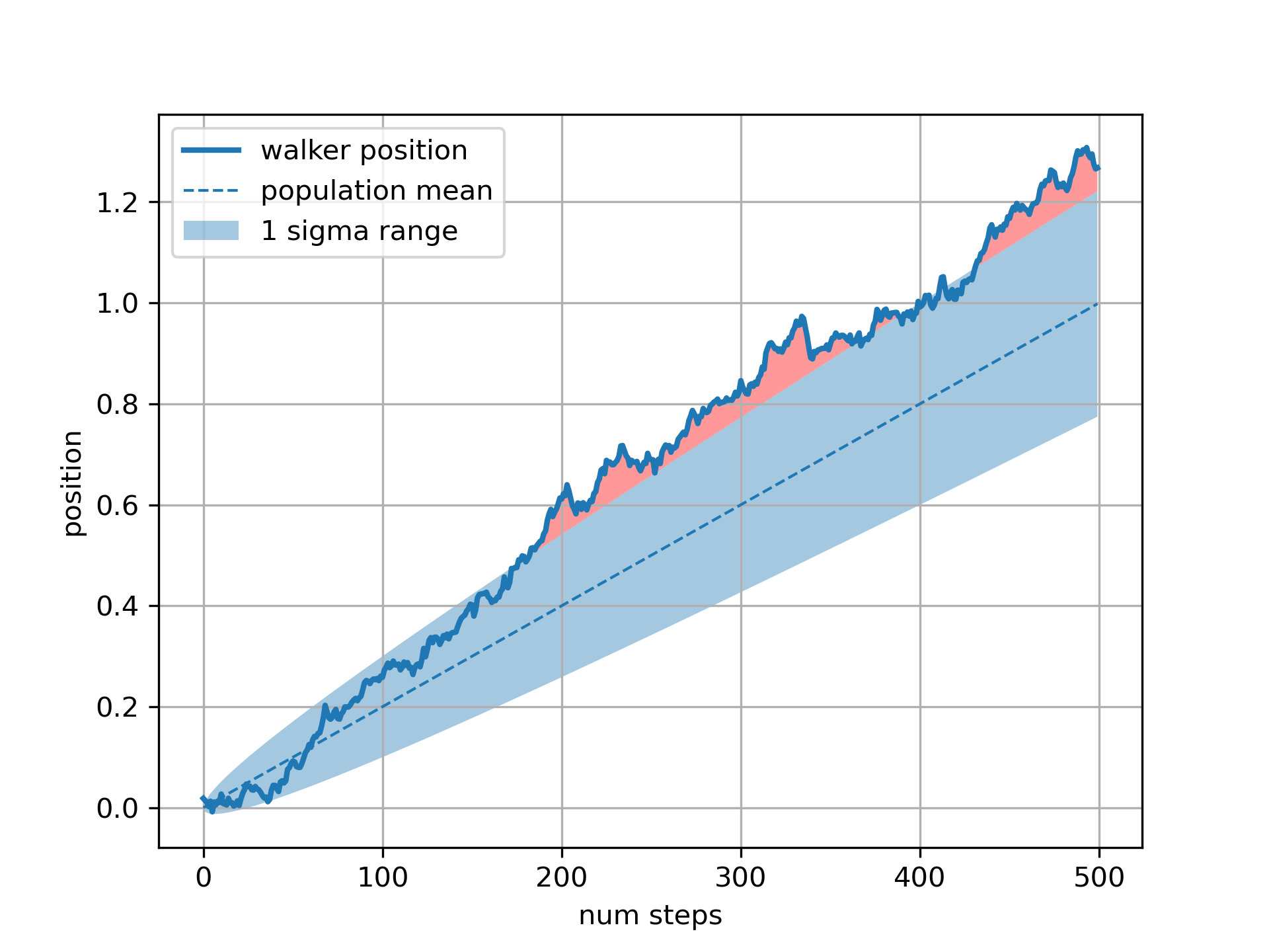
... # The ``where`` keyword argument is very handy for highlighting certain
... # regions of the graph.  ``where`` takes a boolean mask the same length
... # as the x, ymin and ymax arguments, and only fills in the region where
... # the boolean mask is True.  In the example below, we simulate a single
... # random walker and compute the analytic mean and standard deviation of
... # the population positions.  The population mean is shown as the dashed
... # line, and the plus/minus one sigma deviation from the mean is shown
... # as the filled region.  We use the where mask ``X > upper_bound`` to
... # find the region where the walker is outside the one sigma boundary,
... # and shade that region red.
... 
... # Fixing random state for reproducibility
... np.random.seed(1)
... 
... Nsteps = 500
... t = np.arange(Nsteps)
... 
... mu = 0.002
... sigma = 0.01
... 
... # the steps and position
... S = mu + sigma*np.random.randn(Nsteps)
... X = S.cumsum()
... 
... # the 1 sigma upper and lower analytic population bounds
... lower_bound = mu*t - sigma*np.sqrt(t)
... upper_bound = mu*t + sigma*np.sqrt(t)
... 
... fig, ax = plt.subplots(1)
... ax.plot(t, X, lw=2, label='walker position')
... ax.plot(t, mu*t, lw=1, label='population mean', color='C0', ls='--')
... ax.fill_between(t, lower_bound, upper_bound, facecolor='C0', alpha=0.4,
...                 label='1 sigma range')
... ax.legend(loc='upper left')
... 
... # here we use the where argument to only fill the region where the
... # walker is above the population 1 sigma boundary
... ax.fill_between(t, upper_bound, X, where=X > upper_bound, fc='red', alpha=0.4)
... ax.fill_between(t, lower_bound, X, where=X < lower_bound, fc='red', alpha=0.4)
... ax.set_xlabel('num steps')
... ax.set_ylabel('position')
... ax.grid()
... 
... ###############################################################################
... # Another handy use of filled regions is to highlight horizontal or vertical
... # spans of an axes -- for that Matplotlib has the helper functions
... # `~matplotlib.axes.Axes.axhspan` and `~matplotlib.axes.Axes.axvspan`.  See
... # :doc:`/gallery/subplots_axes_and_figures/axhspan_demo`.
... 
... plt.show()
...