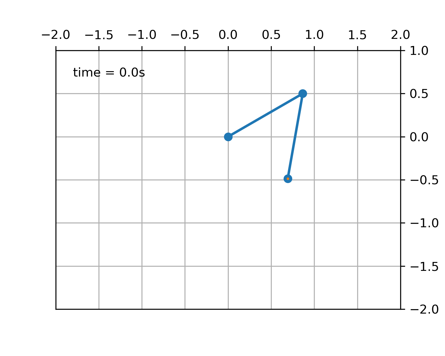
>>> """
===========================
The double pendulum problem
===========================

This animation illustrates the double pendulum problem.

Double pendulum formula translated from the C code at
http://www.physics.usyd.edu.au/~wheat/dpend_html/solve_dpend.c
"""
... 
... from numpy import sin, cos
... import numpy as np
... import matplotlib.pyplot as plt
... import scipy.integrate as integrate
... import matplotlib.animation as animation
... from collections import deque
... 
... G = 9.8  # acceleration due to gravity, in m/s^2
... L1 = 1.0  # length of pendulum 1 in m
... L2 = 1.0  # length of pendulum 2 in m
... L = L1 + L2  # maximal length of the combined pendulum
... M1 = 1.0  # mass of pendulum 1 in kg
... M2 = 1.0  # mass of pendulum 2 in kg
... t_stop = 5  # how many seconds to simulate
... history_len = 500  # how many trajectory points to display
... 
... 
... def derivs(state, t):
... 
...     dydx = np.zeros_like(state)
...     dydx[0] = state[1]
... 
...     delta = state[2] - state[0]
...     den1 = (M1+M2) * L1 - M2 * L1 * cos(delta) * cos(delta)
...     dydx[1] = ((M2 * L1 * state[1] * state[1] * sin(delta) * cos(delta)
...                 + M2 * G * sin(state[2]) * cos(delta)
...                 + M2 * L2 * state[3] * state[3] * sin(delta)
...                 - (M1+M2) * G * sin(state[0]))
...                / den1)
... 
...     dydx[2] = state[3]
... 
...     den2 = (L2/L1) * den1
...     dydx[3] = ((- M2 * L2 * state[3] * state[3] * sin(delta) * cos(delta)
...                 + (M1+M2) * G * sin(state[0]) * cos(delta)
...                 - (M1+M2) * L1 * state[1] * state[1] * sin(delta)
...                 - (M1+M2) * G * sin(state[2]))
...                / den2)
... 
...     return dydx
... 
... # create a time array from 0..t_stop sampled at 0.02 second steps
... dt = 0.02
... t = np.arange(0, t_stop, dt)
... 
... # th1 and th2 are the initial angles (degrees)
... # w10 and w20 are the initial angular velocities (degrees per second)
... th1 = 120.0
... w1 = 0.0
... th2 = -10.0
... w2 = 0.0
... 
... # initial state
... state = np.radians([th1, w1, th2, w2])
... 
... # integrate your ODE using scipy.integrate.
... y = integrate.odeint(derivs, state, t)
... 
... x1 = L1*sin(y[:, 0])
... y1 = -L1*cos(y[:, 0])
... 
... x2 = L2*sin(y[:, 2]) + x1
... y2 = -L2*cos(y[:, 2]) + y1
... 
... fig = plt.figure(figsize=(5, 4))
... ax = fig.add_subplot(autoscale_on=False, xlim=(-L, L), ylim=(-L, 1.))
... ax.set_aspect('equal')
... ax.grid()
... 
... line, = ax.plot([], [], 'o-', lw=2)
... trace, = ax.plot([], [], '.-', lw=1, ms=2)
... time_template = 'time = %.1fs'
... time_text = ax.text(0.05, 0.9, '', transform=ax.transAxes)
... history_x, history_y = deque(maxlen=history_len), deque(maxlen=history_len)
... 
... 
... def animate(i):
...     thisx = [0, x1[i], x2[i]]
...     thisy = [0, y1[i], y2[i]]
... 
...     if i == 0:
...         history_x.clear()
...         history_y.clear()
... 
...     history_x.appendleft(thisx[2])
...     history_y.appendleft(thisy[2])
... 
...     line.set_data(thisx, thisy)
...     trace.set_data(history_x, history_y)
...     time_text.set_text(time_template % (i*dt))
...     return line, trace, time_text
... 
... 
... ani = animation.FuncAnimation(
...     fig, animate, len(y), interval=dt*1000, blit=True)
... plt.show()
...