>>> """
=========================================
Creating a colormap from a list of colors
=========================================
For more detail on creating and manipulating colormaps see
:doc:`/tutorials/colors/colormap-manipulation`.
Creating a :doc:`colormap </tutorials/colors/colormaps>` from a list of colors
can be done with the `.LinearSegmentedColormap.from_list` method. You must
pass a list of RGB tuples that define the mixture of colors from 0 to 1.
Creating custom colormaps
-------------------------
It is also possible to create a custom mapping for a colormap. This is
accomplished by creating dictionary that specifies how the RGB channels
change from one end of the cmap to the other.
Example: suppose you want red to increase from 0 to 1 over the bottom
half, green to do the same over the middle half, and blue over the top
half. Then you would use::
cdict = {'red': ((0.0, 0.0, 0.0),
(0.5, 1.0, 1.0),
(1.0, 1.0, 1.0)),
'green': ((0.0, 0.0, 0.0),
(0.25, 0.0, 0.0),
(0.75, 1.0, 1.0),
(1.0, 1.0, 1.0)),
'blue': ((0.0, 0.0, 0.0),
(0.5, 0.0, 0.0),
(1.0, 1.0, 1.0))}
If, as in this example, there are no discontinuities in the r, g, and b
components, then it is quite simple: the second and third element of
each tuple, above, is the same--call it "y". The first element ("x")
defines interpolation intervals over the full range of 0 to 1, and it
must span that whole range. In other words, the values of x divide the
0-to-1 range into a set of segments, and y gives the end-point color
values for each segment.
Now consider the green. cdict['green'] is saying that for
0 <= x <= 0.25, y is zero; no green.
0.25 < x <= 0.75, y varies linearly from 0 to 1.
x > 0.75, y remains at 1, full green.
If there are discontinuities, then it is a little more complicated.
Label the 3 elements in each row in the cdict entry for a given color as
(x, y0, y1). Then for values of x between x[i] and x[i+1] the color
value is interpolated between y1[i] and y0[i+1].
Going back to the cookbook example, look at cdict['red']; because y0 !=
y1, it is saying that for x from 0 to 0.5, red increases from 0 to 1,
but then it jumps down, so that for x from 0.5 to 1, red increases from
0.7 to 1. Green ramps from 0 to 1 as x goes from 0 to 0.5, then jumps
back to 0, and ramps back to 1 as x goes from 0.5 to 1.::
row i: x y0 y1
/
/
row i+1: x y0 y1
Above is an attempt to show that for x in the range x[i] to x[i+1], the
interpolation is between y1[i] and y0[i+1]. So, y0[0] and y1[-1] are
never used.
"""
... import numpy as np
... import matplotlib as mpl
... import matplotlib.pyplot as plt
... from matplotlib.colors import LinearSegmentedColormap
...
... # Make some illustrative fake data:
...
... x = np.arange(0, np.pi, 0.1)
... y = np.arange(0, 2 * np.pi, 0.1)
... X, Y = np.meshgrid(x, y)
... Z = np.cos(X) * np.sin(Y) * 10
...
...
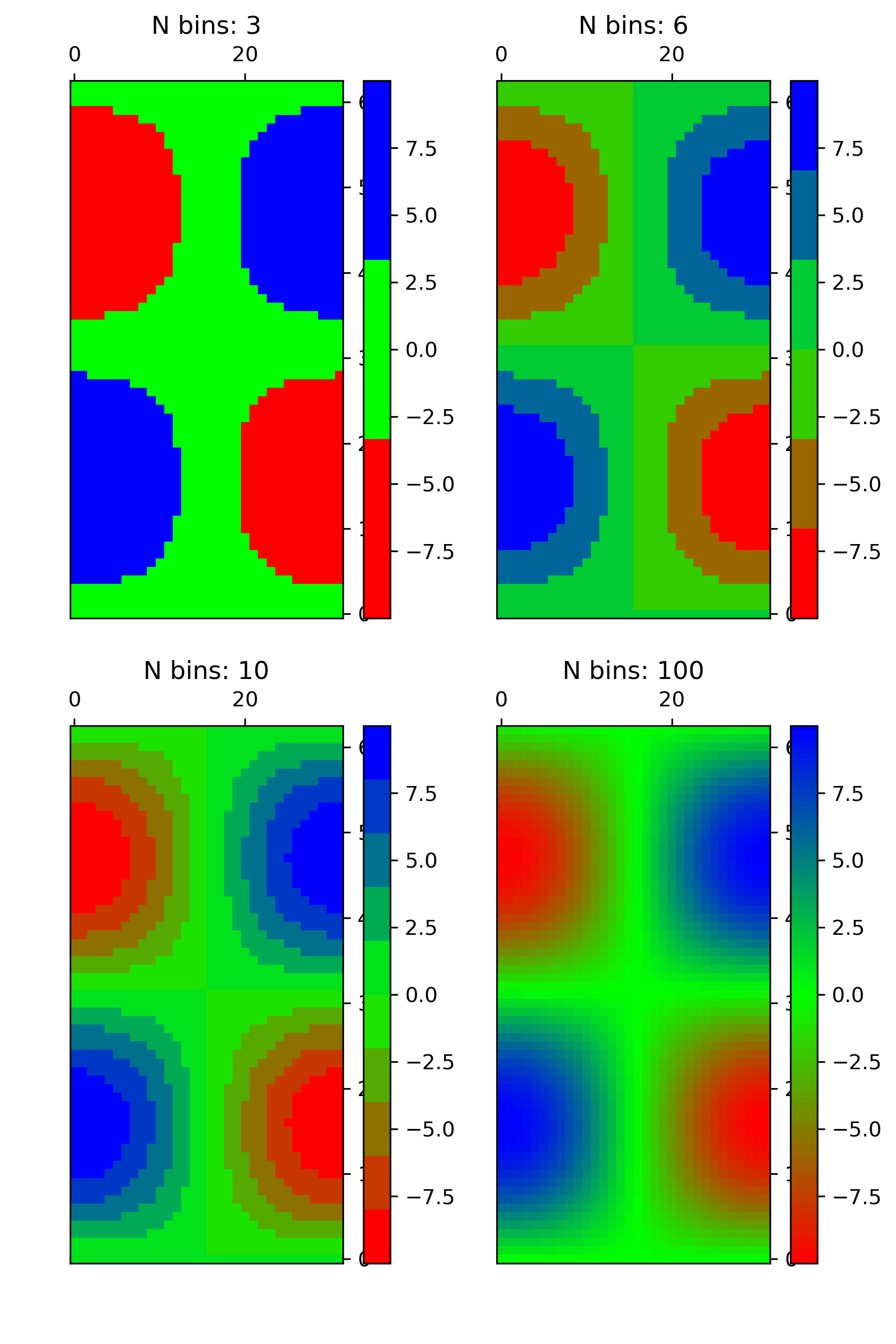
... ###############################################################################
... # --- Colormaps from a list ---
...
... colors = [(1, 0, 0), (0, 1, 0), (0, 0, 1)] # R -> G -> B
... n_bins = [3, 6, 10, 100] # Discretizes the interpolation into bins
... cmap_name = 'my_list'
... fig, axs = plt.subplots(2, 2, figsize=(6, 9))
... fig.subplots_adjust(left=0.02, bottom=0.06, right=0.95, top=0.94, wspace=0.05)
... for n_bin, ax in zip(n_bins, axs.flat):
... # Create the colormap
... cmap = LinearSegmentedColormap.from_list(cmap_name, colors, N=n_bin)
... # Fewer bins will result in "coarser" colomap interpolation
... im = ax.imshow(Z, origin='lower', cmap=cmap)
... ax.set_title("N bins: %s" % n_bin)
... fig.colorbar(im, ax=ax)
...
...
... ###############################################################################
... # --- Custom colormaps ---
...
... cdict1 = {'red': ((0.0, 0.0, 0.0),
... (0.5, 0.0, 0.1),
... (1.0, 1.0, 1.0)),
...
... 'green': ((0.0, 0.0, 0.0),
... (1.0, 0.0, 0.0)),
...
... 'blue': ((0.0, 0.0, 1.0),
... (0.5, 0.1, 0.0),
... (1.0, 0.0, 0.0))
... }
...
... cdict2 = {'red': ((0.0, 0.0, 0.0),
... (0.5, 0.0, 1.0),
... (1.0, 0.1, 1.0)),
...
... 'green': ((0.0, 0.0, 0.0),
... (1.0, 0.0, 0.0)),
...
... 'blue': ((0.0, 0.0, 0.1),
... (0.5, 1.0, 0.0),
... (1.0, 0.0, 0.0))
... }
...
... cdict3 = {'red': ((0.0, 0.0, 0.0),
... (0.25, 0.0, 0.0),
... (0.5, 0.8, 1.0),
... (0.75, 1.0, 1.0),
... (1.0, 0.4, 1.0)),
...
... 'green': ((0.0, 0.0, 0.0),
... (0.25, 0.0, 0.0),
... (0.5, 0.9, 0.9),
... (0.75, 0.0, 0.0),
... (1.0, 0.0, 0.0)),
...
... 'blue': ((0.0, 0.0, 0.4),
... (0.25, 1.0, 1.0),
... (0.5, 1.0, 0.8),
... (0.75, 0.0, 0.0),
... (1.0, 0.0, 0.0))
... }
...
... # Make a modified version of cdict3 with some transparency
... # in the middle of the range.
... cdict4 = {**cdict3,
... 'alpha': ((0.0, 1.0, 1.0),
... # (0.25, 1.0, 1.0),
... (0.5, 0.3, 0.3),
... # (0.75, 1.0, 1.0),
... (1.0, 1.0, 1.0)),
... }
...
...
... ###############################################################################
... # Now we will use this example to illustrate 2 ways of
... # handling custom colormaps.
... # First, the most direct and explicit:
...
... blue_red1 = LinearSegmentedColormap('BlueRed1', cdict1)
...
... ###############################################################################
... # Second, create the map explicitly and register it.
... # Like the first method, this method works with any kind
... # of Colormap, not just
... # a LinearSegmentedColormap:
...
... mpl.colormaps.register(LinearSegmentedColormap('BlueRed2', cdict2))
... mpl.colormaps.register(LinearSegmentedColormap('BlueRed3', cdict3))
... mpl.colormaps.register(LinearSegmentedColormap('BlueRedAlpha', cdict4))
...
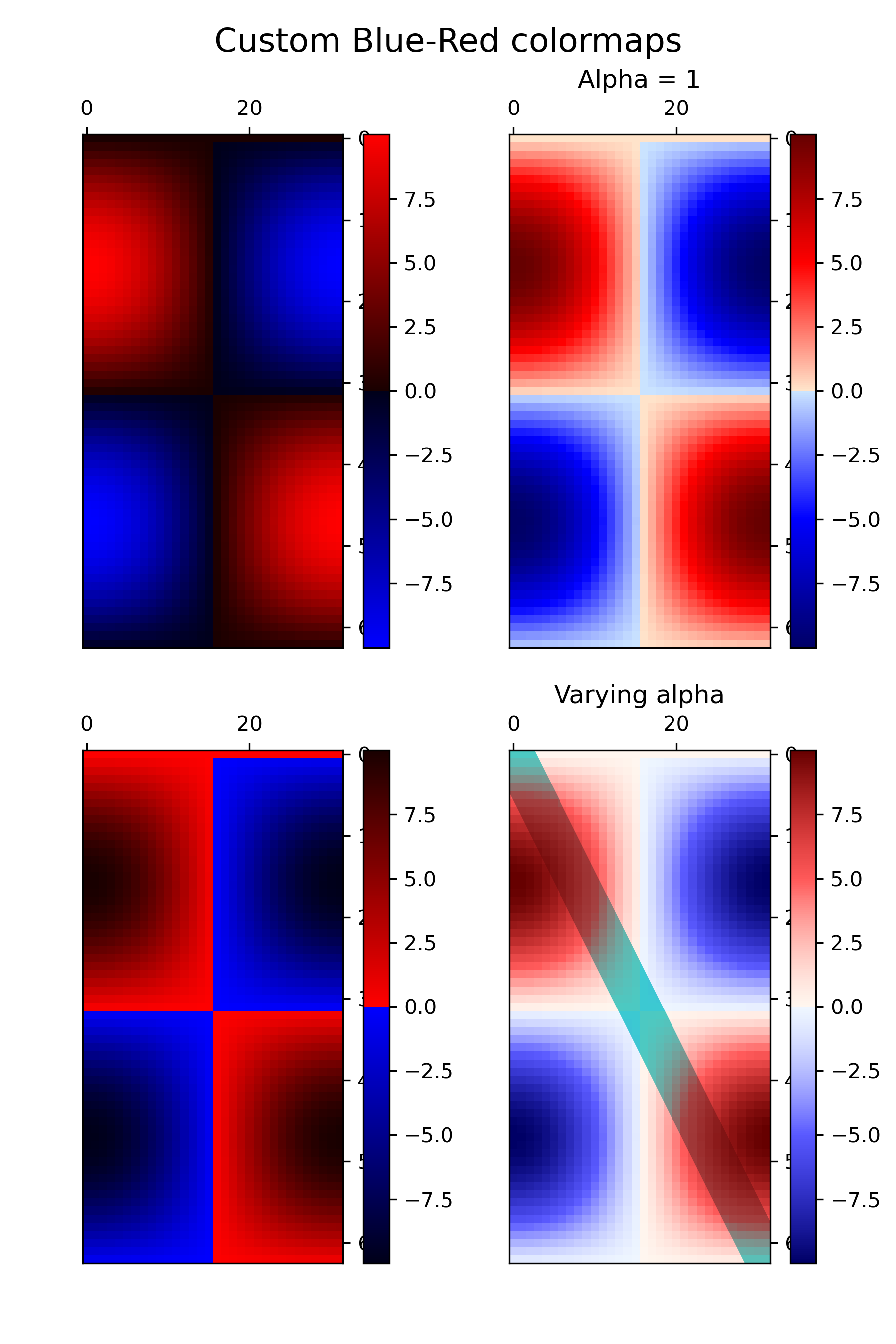
... ###############################################################################
... # Make the figure:
...
... fig, axs = plt.subplots(2, 2, figsize=(6, 9))
... fig.subplots_adjust(left=0.02, bottom=0.06, right=0.95, top=0.94, wspace=0.05)
...
... # Make 4 subplots:
...
... im1 = axs[0, 0].imshow(Z, cmap=blue_red1)
... fig.colorbar(im1, ax=axs[0, 0])
...
... im2 = axs[1, 0].imshow(Z, cmap='BlueRed2')
... fig.colorbar(im2, ax=axs[1, 0])
...
... # Now we will set the third cmap as the default. One would
... # not normally do this in the middle of a script like this;
... # it is done here just to illustrate the method.
...
... plt.rcParams['image.cmap'] = 'BlueRed3'
...
... im3 = axs[0, 1].imshow(Z)
... fig.colorbar(im3, ax=axs[0, 1])
... axs[0, 1].set_title("Alpha = 1")
...
... # Or as yet another variation, we can replace the rcParams
... # specification *before* the imshow with the following *after*
... # imshow.
... # This sets the new default *and* sets the colormap of the last
... # image-like item plotted via pyplot, if any.
... #
...
... # Draw a line with low zorder so it will be behind the image.
... axs[1, 1].plot([0, 10 * np.pi], [0, 20 * np.pi], color='c', lw=20, zorder=-1)
...
... im4 = axs[1, 1].imshow(Z)
... fig.colorbar(im4, ax=axs[1, 1])
...
... # Here it is: changing the colormap for the current image and its
... # colorbar after they have been plotted.
... im4.set_cmap('BlueRedAlpha')
... axs[1, 1].set_title("Varying alpha")
... #
...
... fig.suptitle('Custom Blue-Red colormaps', fontsize=16)
... fig.subplots_adjust(top=0.9)
...
... plt.show()
...
... #############################################################################
... #
... # .. admonition:: References
... #
... # The use of the following functions, methods, classes and modules is shown
... # in this example:
... #
... # - `matplotlib.axes.Axes.imshow` / `matplotlib.pyplot.imshow`
... # - `matplotlib.figure.Figure.colorbar` / `matplotlib.pyplot.colorbar`
... # - `matplotlib.colors`
... # - `matplotlib.colors.LinearSegmentedColormap`
... # - `matplotlib.colors.LinearSegmentedColormap.from_list`
... # - `matplotlib.cm`
... # - `matplotlib.cm.ScalarMappable.set_cmap`
... # - `matplotlib.cm.register_cmap`
...