>>> """
==============================================
Contouring the solution space of optimizations
==============================================

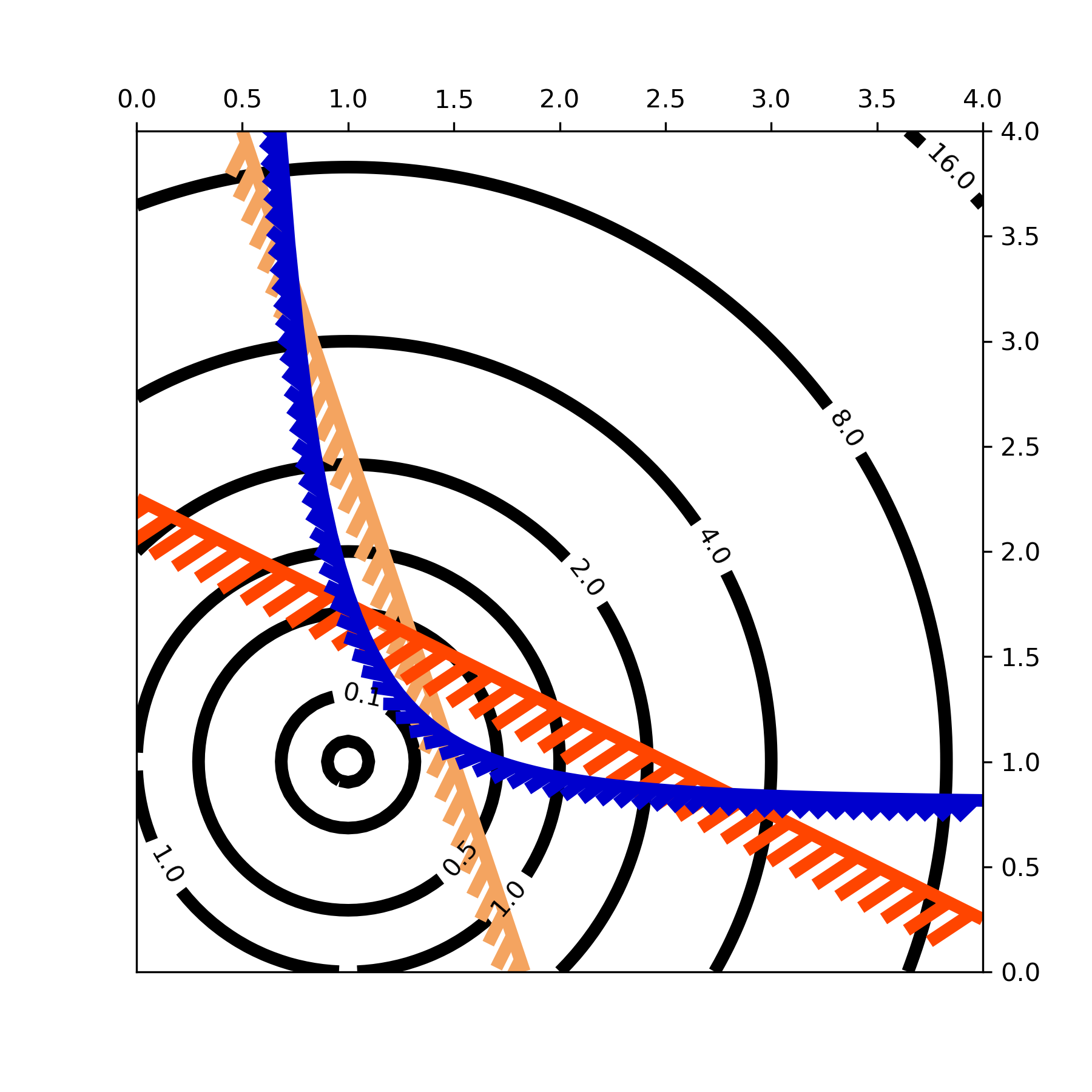
Contour plotting is particularly handy when illustrating the solution
space of optimization problems.  Not only can `.axes.Axes.contour` be
used to represent the topography of the objective function, it can be
used to generate boundary curves of the constraint functions.  The
constraint lines can be drawn with
`~matplotlib.patheffects.TickedStroke` to distinguish the valid and
invalid sides of the constraint boundaries.

`.axes.Axes.contour` generates curves with larger values to the left
of the contour.  The angle parameter is measured zero ahead with
increasing values to the left.  Consequently, when using
`~matplotlib.patheffects.TickedStroke` to illustrate a constraint in
a typical optimization problem, the angle should be set between
zero and 180 degrees.

"""
... 
... import numpy as np
... import matplotlib.pyplot as plt
... from matplotlib import patheffects
... 
... fig, ax = plt.subplots(figsize=(6, 6))
... 
... nx = 101
... ny = 105
... 
... # Set up survey vectors
... xvec = np.linspace(0.001, 4.0, nx)
... yvec = np.linspace(0.001, 4.0, ny)
... 
... # Set up survey matrices.  Design disk loading and gear ratio.
... x1, x2 = np.meshgrid(xvec, yvec)
... 
... # Evaluate some stuff to plot
... obj = x1**2 + x2**2 - 2*x1 - 2*x2 + 2
... g1 = -(3*x1 + x2 - 5.5)
... g2 = -(x1 + 2*x2 - 4.5)
... g3 = 0.8 + x1**-3 - x2
... 
... cntr = ax.contour(x1, x2, obj, [0.01, 0.1, 0.5, 1, 2, 4, 8, 16],
...                   colors='black')
... ax.clabel(cntr, fmt="%2.1f", use_clabeltext=True)
... 
... cg1 = ax.contour(x1, x2, g1, [0], colors='sandybrown')
... plt.setp(cg1.collections,
...          path_effects=[patheffects.withTickedStroke(angle=135)])
... 
... cg2 = ax.contour(x1, x2, g2, [0], colors='orangered')
... plt.setp(cg2.collections,
...          path_effects=[patheffects.withTickedStroke(angle=60, length=2)])
... 
... cg3 = ax.contour(x1, x2, g3, [0], colors='mediumblue')
... plt.setp(cg3.collections,
...          path_effects=[patheffects.withTickedStroke(spacing=7)])
... 
... ax.set_xlim(0, 4)
... ax.set_ylim(0, 4)
... 
... plt.show()
...